Fitting Double Components
Sometimes a emission line is categorized by more than a single line of site emission feature. In this example, we are going to create two Halpha components (and the other usual emission lines in SN3). We will then fit the double components and the other lines.
A very natural question is: how does LUCI fit multiple components?
You will see that the commands are identical to previous fitting commands. The main difference comes from an additional constraint that is imposed on the fit algorithm: if a line appears twice then the velocities of the two lines cannot be equivalent. This is a very light constraint and, thus, doesn’t always work! However, it imposes the least amount of constraints on the fitting algorithm. If you have thoughts on other methods to do this, please let me know!
Let’s start of with the usual slew of commands.
# Imports
import sys
sys.path.insert(0, '/media/carterrhea/carterrhea/SIGNALS/LUCI/')  # Location of Luci
from LUCI.LuciSim import Spectrum
import matplotlib.pyplot as plt
from astropy.io import fits
import numpy as np
import LUCI.LuciFit as lfit
import keras
We now will set the required parameters. You can find a more detailed discussion on how to create synthetic spectra in the example on synthetic spectra!
Let’s first create the single component spectrum
lines = ['Halpha', 'NII6583', 'NII6548', 'SII6716', 'SII6731']
fit_function = 'sincgauss'
ampls = [10, 1, 1, 0.5, 0.45]  # Just randomly choosing these
velocity = 0  # km/s
broadening = 10  # km/s
filter_ = 'SN3'
resolution = 5000
snr = 100
spectrum_axis, spectrum = Spectrum(lines, fit_function, ampls, velocity, broadening, filter_, resolution, snr).create_spectrum()
Now we can add another Halpha line :) To do this, we just need to add an additional line, an additional amplitude, and a different velocity.
lines = ['Halpha']
ampls = [6]  # Just randomly chosen
velocity = 50  # km/s

spectrum_axis2, spectrum2 = Spectrum(lines, fit_function, ampls, velocity, broadening, filter_, resolution, snr).create_spectrum()

# Add them together
spectrum += spectrum2
Now we can go about fitting this spectrum. To do this, we have to do the interpolation on the reference spectrum used for our machine learning algorithm manually. Please note that this is all done internally in LUCI normally.
# Machine Learning Reference Spectrum
ref_spec = fits.open('/media/carterrhea/carterrhea/SIGNALS/LUCI/ML/Reference-Spectrum-R5000-SN3.fits')[1].data
channel = []
counts = []
for chan in ref_spec:  # Only want SN3 region
  channel.append(chan[0])
  counts.append(np.real(chan[1]))
min_ = np.argmin(np.abs(np.array(channel)-14700))
max_ = np.argmin(np.abs(np.array(channel)-15600))
wavenumbers_syn = channel[min_:max_]
f = interpolate.interp1d(spectrum_axis, spectrum, kind='slinear')
sky_corr = (f(wavenumbers_syn))
sky_corr_scale = np.max(sky_corr)
sky_corr = sky_corr/sky_corr_scale
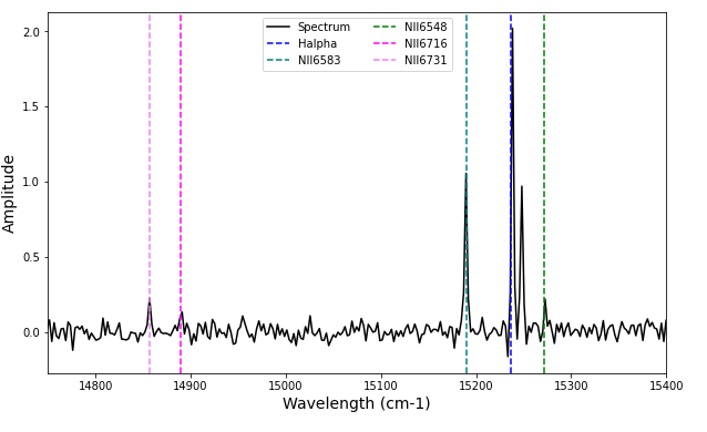
Let’s plot this
plt.figure(figsize=(10,6))
plt.plot(spectrum_axis, spectrum, color='black', label='Spectrum')
plt.xlim(14750, 15400)
plt.xlabel('Wavelength (cm-1)', fontsize=14)
plt.ylabel('Amplitude', fontsize=14)
plt.axvline(1e7/656.3, label='Halpha', color='blue', linestyle='--')
plt.axvline(1e7/658.3, label='NII6583', color='teal', linestyle='--')
plt.axvline(1e7/654.8, label='NII6548', color='green', linestyle='--')
plt.axvline(1e7/671.6, label='NII6716', color='magenta', linestyle='--')
plt.axvline(1e7/673.1, label='NII6731', color='violet', linestyle='--')
plt.legend(ncol=2)
plt.show()
We can now fit the spectrum. After much testing of fitting double components, I find that setting the Bayesian analysis is really helpful here. Without setting it, the results are not always correct (there is some stochasticity in the fitting algorithm). On the other hand, the Bayesian approach seems to always achieve the correct values. If you find any descrepencies at all, please let me know!
fit = lfit.Fit(spectrum, spectrum_axis, wavenumbers_syn, 'sincgauss',
               ['Halpha', 'NII6583', 'NII6548','SII6716', 'SII6731', 'Halpha'],
               [1,1,1,1,1,2], [1,1,1,1,1,2],
               keras.models.load_model('/media/carterrhea/carterrhea/SIGNALS/LUCI/ML/R5000-PREDICTOR-I-SN3')
               bayes_bool=True
             )
fit_dict = fit.fit()
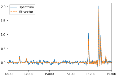
And let’s visualize that fit..
plt.plot(spectrum_axis, spectrum, label='spectrum')
plt.plot(spectrum_axis, fit_dict['fit_vector'], label='fit vector', linestyle='--')
plt.xlim(14800, 15300)
plt.legend()