Example of fitting regions in NGC6888
In this notebook, we go through fitting two regions of NGC 6888. This notebook exists for the sole purpose of demonstrating LUCI’s prowess at fitting regions :)
This notebook thus assumes that you have already gone through the tutorials.
# Imports
import sys
sys.path.insert(0, '/media/carterrhea/carterrhea/SIGNALS/LUCI/')  # Location of Luci
from LuciBase import Luci
import LUCI.LuciPlotting as lplt
We now will set the required parameters. We are also going to be using our machine learning algorithm to get the initial guesses.
#Set Parameters
# Using Machine Learning Algorithm for Initial Guess
Luci_path = '/home/carterrhea/Documents/LUCI/'
cube_dir = '/home/carterrhea/Documents/NGC6888'  # Path to data cube
cube_name = 'NGC6888_SN3'  # don't add .hdf5 extension
object_name = 'NGC6888'
redshift = 0.0
resolution = 5000
We intialize our LUCI object
# Create Luci object
cube = Luci(Luci_path, cube_dir+'/'+cube_name, cube_dir, object_name, redshift, resolution)
Picking the regions
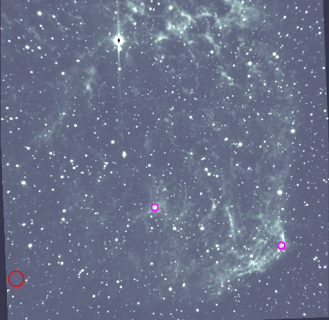
Now let’s take a quick look at the deep image to decide the regions we will fit.

I’ve highlighted the background red in green and the two fit regions in magenta. Region 1 is near the right edge of the image and reigon 2 is at the center3.
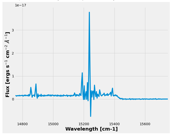
Let’s take a look at the background
bkg_axis, bkg_sky = cube.extract_spectrum_region(cube_dir+'/bkg.reg', mean=True)  # We use mean=True to take the mean of the emission in the region instead of the sum
lplt.plot_spectrum(bkg_axis, bkg_sky)

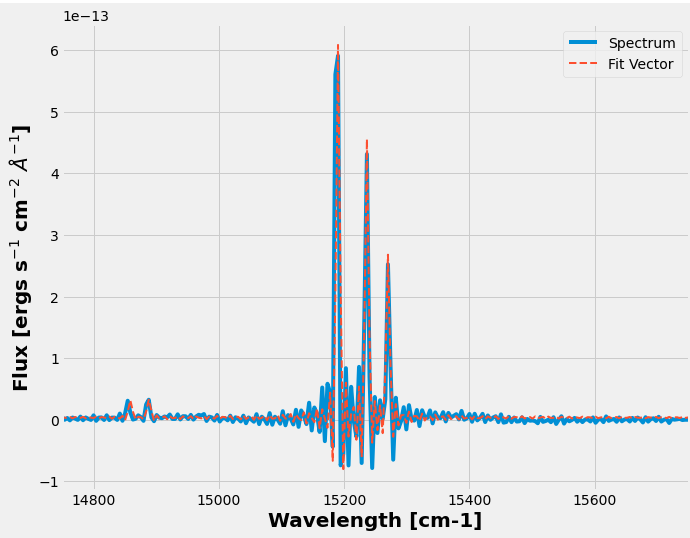
Now we can define our fit region and fit it!
axis, sky, fit_dict = cube.fit_spectrum_region(
                            ['NII6548', 'Halpha', 'NII6583', 'SII6716', 'SII6731'],
                            'sincgauss',
                            [1,1,1,1,1], [1,1,1,1,1],
                            region=cube_dir+'/region1.reg', bkg=bkg_sky,
                            bayes_bool=False)
lplt.plot_fit(axis, sky, fit_dict['fit_vector'])
And let’s see how this looks

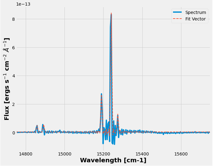
axis, sky, fit_dict = cube.fit_spectrum_region(
                            ['NII6548', 'Halpha', 'NII6583', 'SII6716', 'SII6731'],
                            'sincgauss',
                            [1,1,1,1,1], [1,1,1,1,1],
                            region=cube_dir+'/region2.reg', bkg=bkg_sky,
                            bayes_bool=False)
lplt.plot_fit(axis, sky, fit_dict['fit_vector'])
And let’s see how this looks

Overall, these fits look pretty great :D