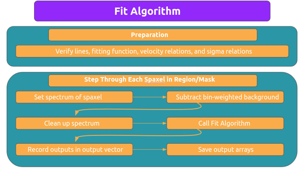
Fitting Algorithm

This section contains the functions used to fit emission lines.

Fitting Functions

class LUCI.LuciFit.Fit(spectrum, axis, wavenumbers_syn, model_type='sinc', lines=['Halpha'], vel_rel=[1], sigma_rel=[1], ML_bool=True, trans_filter=None, theta=0, delta_x=2943, n_steps=842, zpd_index=169, filter='SN3', bayes_bool=False, bayes_method='emcee', uncertainty_bool=False, mdn=False, nii_cons=True, sky_lines=None, sky_lines_scale=None, initial_values=[False], spec_min=None, spec_max=None, obj_redshift=0.0, n_stoch=1, resolution=1000, Luci_path=None)

Class that defines the functions necessary for the modelling aspect. This includes the gaussian fit functions, the prior definitions, the log likelihood, and the definition of the posterior (log likelihood times prior).

All the functions (gauss, sinc, and sincgauss) are stored in LuciFuncitons.py.

All functions for calculating the velocity, broadening, and flux are in ‘LuciFitParameters.py’.

All the functions for Bayesian Inference with the exception of the fit call are in ‘LuciBayesian.py’.

The returned axis is the redshifted axis.

If the initial_values argument is passed, then the fit algorithm will use these values [velocity, broadening] as the initial conditions for the fit instead of the machine learning algorithm. See example ‘initial_values’ for more details on the implementation.

NII_constraints()

Enforce the constraint that the NII6548 lines has an amplitude that is 1/3 the amplitude of NII6583.

Returns:

Constraint on NII doublet relative amplitudes

amplitude_constraint()

Constraint that requires the amplitude of the line be positive

apply_transmission()

Apply transmission curve on the spectra according to un-redshifted axis. This is done before we interpolate onto the wavenumbers_syn so that the axis align properly. Note – the values of the x-axis are not important for this division since we have already interpolated the transition filter vector over the UNSHIFTED spectral axis.

calc_chisquare(fit_vector, init_spectrum, init_errors, n_dof)

Calculate reduced chi 2

Parameters:

• fit_vector – Spectrum obtained from fit

• init_spectrum – Observed spectrum

• init_errors – Errors on observed spectrum

• n_dof – Number of degrees of freedom

Returns:

Chi squared value chi2dof: Reduced chi squared value

Return type:

chi2

calc_sinc_width()

Calculate sinc width of the sincgauss function

calculate_correction()

Calculate correction factor based of interferometric angle. This is used to correct the broadening

calculate_noise()

Calculate noise level in spectrum. We assume the noise is homogenous across the spectrum. We estimate it by taking a region outside of the filter and calculating the standard deviation in that region. We use the normalized spectrum since that is what is passed to the fit function.

calculate_params()

Calculate the amplitude, position, and sigma of the line. These values are calculated using the scipy.optimize.minimize function. This is called on the log likelood previously described. The minimization algorithm uses the SLSQP optimization implementation. We have applied standard bounds in order to speed up the fitting. We also apply the fit on the normalized spectrum. We then correct the flux by un-normalizing the spectrum.

check_fitting_model()

This function checks to see that the model provided is in the available options Return: Nothing if the user provides an appropriate fitting model Else it will throw an error

check_lengths()

This function checks to see that the length of the sigma_rel and vel_rel arguments are correct Return: Nothing if the user provides appropriate length Else it will throw an error

check_lines()

This function checks to see that the lines provided are in the available options Return: Nothing if the user provides appropriate lines Else it will throw an error

cont_estimate(sigma_level=3)

TODO: Test

Function to estimate the continuum level. We use a sigma clipping algorithm over the(mu_vel/SPEED_OF_LIGHT)*line_dict[line[ct]] + line_dict[line[ct]] restricted axis/spectrum to effectively ignore emission lines. Therefore, we are left with the continuum. We take the minimum value of this continuum as the initial guess.

Parameters:

sigma_level – Sigma level to clip (Default=3)

Returns:

Initial guess for continuum

estimate_priors_ML(mdn=True)

Apply machine learning algorithm on spectrum in order to estimate the velocity. The spectrum fed into this method must be interpolated already onto the reference spectrum axis AND normalized as described in Rhea et al. 2020a. :param mdn: Boolean to use MDN or not (default True)

Returns:

Updates self.vel_ml

fit(sky_line=False)

Primary function call for a spectrum. This will estimate the velocity using our machine learning algorithm described in Rhea et al. 2020a. Then we will fit our lines using scipy.optimize.minimize.

Parameters:

sky_line – Boolean to fit sky lines (default False)

Returns:

{“fit_vector”: Fitted spectrum, “velocity”: Velocity of the line in km/s (float), “broadening”: Velocity Dispersion of the line in km/s (float)}

Return type:

dictionary of parameters returned by the fit. The dictionary has the following form

fit_Bayes()

Apply Bayesian MCMC run to constrain the parameters after solving

interpolate_spectrum()

Interpolate Spectrum given the wavelength axis of reference spectrum. Then normalize the spectrum so that the max value equals 1

Returns:

Populates self.spectrum_interpolated, self.spectrum_scale, and self.spectrum_interp_norm.

line_vals_estimate(line_name)

TODO: Test

Function to estimate the position and amplitude of a given line.

Parameters:

line_name – Name of model. Available options are ‘Halpha’, ‘NII6548’, ‘NII6543’, ‘SII6716’, ‘SII6731’

Returns:

Estimated line amplitude in units of cm-1 (line_amp_est) and estimate line position in units of cm-1 (line_pos_est)

log_likelihood(theta)

Calculate log likelihood function evaluated given parameters on spectral axis

Parameters:

theta –

List of parameters for all the models in the following order

[amplitude, line location, sigma, continuum constant]

The continuum constant is always the last argument regardless of the number of lines being modeled

Returns:

Value of log likelihood

multiple_component_vel_constraint()

Constraint that requires each line have a different position.

restrict_wavelength()

Restrict the wavelength range of the fit so that the fit only occurs over the central regions of the spectra. We do this so that the continuum is properly calculated.

sigma_constraints()

Set up constraints for sigma values before fitting line :returns: Dictionary describing constraints

vel_constraints()

Set up constraints for velocity values before fitting line :returns: Dictionary describing constraints