Fit Single Spectrum
In this example, we will extract a region of M33 Field 7 SN3 and fit is using LUCI. This is a very basic example.
# Imports
import sys
sys.path.insert(0, '/media/carterrhea/carterrhea/SIGNALS/LUCI/')  # Location of Luci
from LuciBase import Luci
import LUCI.LuciPlotting as lplt
We now will set the required parameters. W
# Initialize paths and set parameters
Luci_path = '/home/carterrhea/Documents/LUCI/'
cube_dir = '/export/home/carterrhea/M33'  # Path to data cube
#cube_dir = '/mnt/carterrhea/carterrhea/NGC628'  # Full path to data cube (example 2)
cube_name = 'M33_SN3'  # don't add .hdf5 extension
object_name = 'M33'
filter_name = 'SN3'
redshift = -0.0006  # Redshift of object
resolution = 5000
We intialize our LUCI object
# Create Luci object
cube = Luci(Luci_path, cube_dir+'/'+cube_name, cube_dir, object_name, redshift, resolution)
Let’s extract a background region and take a look at it. The background region is defined in a ds9 region file called Luci_path/Examples/regions/bkg_M33.reg.
bkg_axis, bkg_sky = cube.extract_spectrum_region(Luci_path+'Examples/regions/bkg_M33.reg', mean=True)
  lplt.plot_spectrum(bkg_axis, bkg_sky)
Now we can define our fit region and fit it!
axis, sky, fit_dict = cube.fit_spectrum_region(
                                    ['NII6548', 'Halpha', 'NII6583'],
                                    'sincgauss',
                                    [1,1,1], [1,1,1],
                                    region=Luci_path+'Examples/regions/M33_reg1.reg',
                                    bkg=bkg_sky)
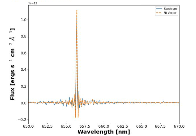
lplt.plot_fit(axis, sky, fit_dict['fit_vector'], units='nm')
plt.xlim(650, 670)
And let’s see how this looks
