Example Freeze
How to use LUCI with frozen parameters
In this example we will go through how to fit a spectrum with frozen velocity and broadening parameters. This may be useful if you want to say fit the Halpha + NII complex to calculate the velocity and broadening of the gas – then you can use these values to constrain a fit on the SII doublet which is frequently weaker.
For this particular example, we will be using the Field 7 of M33 and fitting twice: with and without frozen parameters.
This example can be found as a jupyter notebook in “LUCI/Examples/SN3_freeze.ipynb”.
# Imports
import sys
import numpy as np
sys.path.insert(0, '/home/carterrhea/Documents/LUCI/')  # Location of Luci
from LuciBase import Luci
Inputs
We simply need to load our LUCI cube like usual :) So we start by defining the path, the name of the cube, the name of the object, the resolution (which isn’t actually used here), and the redshift.
Luci_path = '/home/carterrhea/Documents/LUCI/'
cube_dir = '/mnt/carterrhea/carterrhea/M33'  # Path to data cube
cube_name = 'M33_Field7_SN3.merged.cm1.1.0'  # don't add .hdf5 extension
object_name = 'M33_Field7'
redshift = -0.0006  # Redshift of M33
resolution = 5000
As usual we will extract a background
bkg_axis, bkg_sky = cube.extract_spectrum_region(cube_dir+'/bkg.reg', mean=True)  # We use mean=True to take the mean of the emission in the region instead of the sum
lplt.plot_spectrum(bkg_axis, bkg_sky)
Now let’s go ahead and fit the Halpha complex (i.e. Halpha and NII-doublet). We will use the velocity and broadening values found here to fit the SII-doublet.
vel_map, broad_map, flux_map, ampls_map = cube.fit_cube(['Halpha', 'NII6583', 'NII6548'], 'sincgauss',
                                                    [1,1,1], [1,1,1],
                                                    1200, 1350, 1700, 1900,
                                                    bkg=bkg_sky, binning=1,
                                                    uncertainty_bool=False, n_threads=1
                                                   )
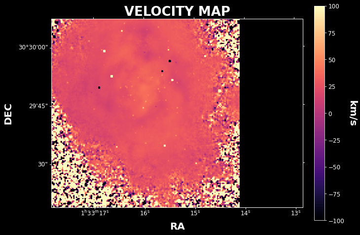
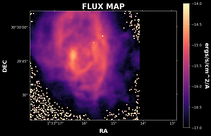
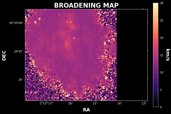
Let’s take a look at our flux, velocity, and broadening maps.
lplt.plot_map(flux_map[:,:,0], 'flux', cube_dir, cube.header, clims=[-17, -14])
lplt.plot_map(vel_map[:,:,0], 'velocity', cube_dir, cube.header, clims=[-100,100])

lplt.plot_map(broad_map[:,:,0], 'broadening', cube_dir, cube.header, clims=[0,30])
Now let’s fit the SII-doublet using the previously calculated velocity and broadening as constraints.
vel_map_fr, broad_map_fr, flux_map_fr, ampls_fr = cube.fit_cube(["SII6716", "SII6731"], 'sincgauss',
                                                    [1,1], [1,1],
                                                    1200, 1350, 1700, 1900,
                                                    bkg=bkg_sky, binning=1,
                                                    uncertainty_bool=False, n_threads=1,
                                                    initial_values=[vel_map[:,:,0], broad_map[:,:,0]]
                                                   )
And we can see that the velocity is in fact being held constant by checking out the resulting velocity map!
lplt.plot_map(vel_map_fr[:,:,0], 'velocity', cube_dir, cube.header, clims=[-100,100])