Example Mask

You can find the data used in this tutorial at the CADC database ([http://www.cadc-ccda.hia-iha.nrc-cnrc.gc.ca/en/search](http://www.cadc-ccda.hia-iha.nrc-cnrc.gc.ca/en/search)) searching for M33_FIELD7 SN1.

# Imports
import sys
sys.path.insert(0, '/media/carterrhea/carterrhea/SIGNALS/LUCI/')  # Location of Luci
from LuciBase import Luci
import LUCI.LuciPlotting as lplt

We now will set the required parameters. We are also going to be using our machine learning algorithm to get the initial guesses.

#Set Parameters
# Using Machine Learning Algorithm for Initial Guess
Luci_path = '/media/carterrhea/carterrhea/SIGNALS/LUCI/'
cube_dir = '/media/carterrhea/carterrhea/M33'  # Path to data cube
cube_name = 'M33_Field7_SN1.merged.cm1.1.0'  # don't add .hdf5 extension
object_name = 'M33_Field7_SN1'
redshift = -0.0006  # Redshift of M33
resolution = 5000

We intialize our LUCI object

# Create Luci object
cube = Luci(Luci_path, cube_dir+'/'+cube_name, cube_dir, object_name, redshift, resolution)

The output will look something like this:

Make Mask

Now we will examine the deep image, choose a region to make a mask out of, and make the mask in numpy.

Please note that you can make a mask any way you would like! Just be sure that the mask that you pass to LUCI for fitting is a numpy boolean array.

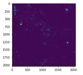
# Create Deep Image
cube.create_deep_image()
plt.imshow(cube.deep_image)
plt.clim(1e-4*np.max(cube.deep_image), 2e-3*np.max(cube.deep_image))
plt.colorbar()

.. image:: M33_Field7_SN1_Deep.png
    :alt: SN1 Field 7 M33 Deep image

We are going to mask out the regions where the deep image value is less than 3e-16.

mask = np.ma.masked_where(cube.deep_image > 3e-16, cube.deep_image).mask

Let us visualize the mask. The regions that are yellow are unmasked regions.

Fitting

Now we will use are mask in a fit!

Let’s extract a background region. The background region is defined in a ds9 region file.

bkg_axis, bkg_sky = cube.extract_spectrum_region(cube_dir+'/bkg.reg', mean=True)  # We use mean=True to take the mean of the emission in the region instead of the sum
plt.plot(bkg_axis, bkg_sky)

# Fit!
vel_map, broad_map, flux_map, chi2_fits, mask = cube.fit_region(['OII3726', 'OII3729'], 'gaussian', [1, 1], [1, 1], mask, bkg=bkg_sky, binning=2)

The output should look something like this:

The number is the number of pixels fitted.

Let’s take a look at the flux map.

lplt.plot_map(flux_map[:,:,0], 'flux', cube_dir, cube.header, clims=[1e-20, 1e-18])

And let’s see what this looks like!

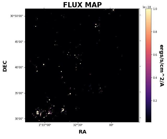
Clearly, this example isn’t beautiful, but we have shown how to use the mask!