How LUCI Works

LUCI is a general purpose line fitting pipeline designed to unveil the inner workings of how fits of SITELLE IFU datacubes are calculated. In this section, I will explain what we are trying to calculate, how it is calculated, and how you can personalize the fits.

What we calculate

The three primary quantities of interest are the amplitude of the line, the position of the line (often described as the velocity and quoted in km/s), and the broadening of the line (often described as the velocity dispersion).

Velocity

The velocity of a line is calculated using the following equation: $v [km/s] = c [km/s] * \Delta \lambda$

c is the speed of light in kilometers per second. Delta lambda is the shift of the measured line. Although the line position is calculated in units of [cm-1], we translate it into nanometers since $\lambda [nm] = \frac{1e7}{\lambda[cm-1]}$ . $\Delta \lambda = (line\_pos[nm]-line\_ref[nm])/line\_ref[nm]$

where $line\_ref$ is the natural position of the line (for example; $line\_ref=656.28 nm$ for Halpha.)

Velocity Dispersion

The velocity dispersion of a line is calculated using the following equation: \Delta v = \frac{3e5 [km/s] * \sigma}{v [km/s]}

where $\sigma$ is the calculated width of a the fitted Gaussian.

Flux

Similarly, we define the flux for each fitting function as the following:

Flux for a Gaussian Function:

$Flux [erg/s/cm^2/Ang] = \sqrt{2\pi}p_0p_2$

Flux for a Sinc Function:

$Flux [erg/s/cm^2/Ang] = \pi p_0p_2$

Flux for a SincGauss Function:

$Flux [erg/s/cm^2/Ang] = \text{coeff} * p_0\frac{\sqrt{2\pi}p_2}{erf(\frac{p_2}{\sqrt{2}\sigma})}$

Note that $text{coeff}=frac{1.20671}{pi*FWHM_COEFF}$ where the FWHM_COEFF equals $2sqrt{2log{2}}, the $pi$ is there because of the sinc function’s definition, and the 1.20671 is the factor used to go between FWHM and sigma.

How we calculate

Once we have a spectrum, we do two things: we normalize the spectrum by the maximum amplitude and we apply a redshift correction (wavelength = wavelength*(1+redshift)). We do this primarily to constrain the velocity to be between -500 and 500 km/s. This allows our machine learning technique to obtain better initial guess estimates.

Initial Guess

Having a good initial guess is crucial for the success (and speed) of the fitting algorithm. In order to obtain a good initial guess for the fit parameters (line amplitude, line position, and line broadening), we apply a machine learning technique described in Rhea et al. 2020a (disclosure: the author of this code is also the author of this paper). The method uses pre-trained convolutional neural networks to estimate the velocity and broadening of the line in km/s. These are then translated into the line position and broadening. Next, the amplitude is taken as the height of the line corresponding to the shifted line position. We note that the machine learning model has only been trained to obtain velocities between -500 and 500 km/s. Similarly, the model was trained to obtain broadening values between 10 and 200 km/s. You can find more information on this at https://sitelle-signals.github.io/Pamplemousse/index.html <https://sitelle-signals.github.io/Pamplemousse/index.html>. We estimate the amplitude by taking the maximum value of spectrum corresponding to the estimated position plus or minus 2 channels.

Since we understand that machine learning is not everyone’s cup of tea, we have an alternative method to calculate the initial guesses.

Fitting Function

The fitting function utilizes scipy.optimize.minimize. Currently, we are using the trust-constr <https://docs.scipy.org/doc/scipy/reference/optimize.minimize-trustconstr.html> optimization algorithm. Before fitting the spectrum, we normalize the spectrum by the maximum amplitude – this makes the fitting process simpler. The fit returns the amplitude of the line (which we then scale to be correct for the un-normalized spectrum), the velocity in km/s, and the velocity dispersion in km/s. If the user chooses, the line velocities and velocity dispersions can be coupled. Additionally, we automatically include the constraint on the NII-doublet flux ratio (setting NII_6583 = 3*NII_6548) using the nii_cons boolean. This can be changed by adding nii_cons=False as an argument to any of the fitting functions.

Available Models

We have implemented three functions: gaussian, sinc, and sincgauss.

Gaussian

We assume a standard form of a Gaussian: $p_0*exp{(-(x-p_1)**2)/(2*p_2**2)}$

We solve for p_0, p_1, and p_2 (x is the wavelength channel and is thus provided). $p_0$ is the amplitude, $p_1$ is the position of the line, and $p_2$ is the broadening.

Sinc

We adopt the following form $u=(x-p_1)/p_2$ $p_0*sinc(\pi*u)/(\pi*u)$

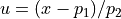
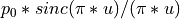
Note that $p_2$ is FIXED for the sinc function as 1/(2*MPD) (where MPD is the maximum path difference).

SincGauss

$p_0*exp(-b*^2)*((erf(a-i*b)+erf(a+i*b))/(2*erf(a)))$

where $a = p_2/(\sqrt{2}*\sigma)$ $b = (x-p_1)/(\sqrt{2}*\sigma)$

We also have the Dawson integral calculation of the sincgauss function:

$p_0*( (dawson(ai+b)exp(2iab) + dawson(ai-b)exp(-2iab)) / 2*dawson(ai) )$

where sigma is 1/(2*MPD).

Therefore, when using a sincgauss, we have to calculate the MPD. We can adopt the following definition: $MPD = \cos{\theta}\delta_x N$ where $\cos{\theta}$ is the cosine angle defined as $\cos{\theta} = \frac{\lambda_{ref}}{\lambda_{ij}}$ . $\lambda_{ref}$ is the wavelength of the calibration laser and $\lambda_{ij}$ is the measured calibration wavelength of a given pixel (thus $\theta$ is a function of the pixel).

Also note that we divide the sinc width ( $p_2$ ) by $\pi$ based on our definition of the sinc width above.

If you are interested in the broadening, we strongly suggest you use the sincgauss function :)

Transmission

We take into account the transmission of the SITTELLE filters (SN1, SN2, and SN3). We take the true transmission as the mean of the transmission at different filter angles; the raw data can be found [here](https://www.cfht.hawaii.edu/Instruments/Sitelle/SITELLE_filters.php). The transmission is then applied to the spectrum in the following manner: if the transmission is above 0.5, then we multiply the spectrum by the transmission percentage. Otherwise, we set it to zero. Note that we calculate the noise before applying the transmission.