Fit Single Region
In this example, we are going to fit a single region of the NGC 6946 data cube. You can download the example data using the following command:
wget https://ws.cadc-ccda.hia-iha.nrc-cnrc.gc.ca/data/pub/CFHT/2307000z.hdf5?RUNID=xc9le6u8llecp7fp
We will read in the data as usual using a LUCI cube object. We then will extract a background region and plot it. We will then extract a spectrum from a square region around 1357<x<1367 and 608<y<618. Finally, we use the LuciFit Fit object to fit the region.
# Imports
import sys
sys.path.insert(0, '/media/carterrhea/carterrhea/SIGNALS/LUCI/')  # Location of Luci
from LuciBase import Luci
import LUCI.LuciPlotting as lplt
import matplotlib.pyplot as plt
import LUCI.LuciFit as lfit
from astropy.io import fits
import numpy as np
import keras
We now will set the required parameters. We are also going to be using our machine learning algorithm to get the initial guesses.
#Set Parameters
# Using Machine Learning Algorithm for Initial Guess
Luci_path = '/home/carterrhea/Documents/LUCI/'
cube_dir = '/home/carterrhea/Documents/LUCI_test'  # Path to data cube
cube_name = 'NGC6946_SN3.merged.cm1.1.0'  # don't add .hdf5 extension
object_name = 'NGC6946'
redshift = 0.000133
resolution = 1000 # The actual resolution is 400, but we don't have machine learning algorithms for that resolution, so we use 1000
We intialize our LUCI object
# Create Luci object
cube = Luci(Luci_path, cube_dir+'/'+cube_name, cube_dir, object_name, redshift, resolution)
Let’s extract and visualize a background region we defined in ds9:
# Extract and visualize background
bkg_axis, bkg_sky = cube.extract_spectrum_region(cube_dir+'/bkg.reg', mean=True)  # We use mean=True to take the mean of the emission in the region instead of the sum
plt.plot(bkg_axis, bkg_sky)

.. image:: example-single-fit-background.png
    :alt: Background output
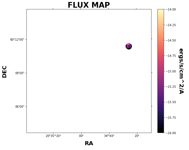
We now fit our region
# fit region
velocity_map, broadening_map, flux_map, chi2_map, mask = cube.fit_region(['OII3726', 'OII3729'], 'gaussian', [1,1], [1,1],
        region=cube_dir+'/reg1.reg', bkg=bkg_sky)
And let’s check out what this looks like.
lplt.plot_map(np.log10(flux_map[:,:,0]), 'flux', cube_dir, cube.header, clims=[-17, -15])