Extract Slices
In this notebook, we will look at how you can use LUCI to extract the channels from your datacube corresponding to a certain emission line! This can be useful if you simply want to see what a channel in the cube looks like.
We currently allow a user to extract the following lines:
‘Halpha’: 656.280, ‘NII6583’: 658.341, ‘NII6548’: 654.803, ‘SII6716’: 671.647, ‘SII6731’: 673.085, ‘OII3726’: 372.603, ‘OII3729’: 372.882, ‘OIII4959’: 495.891, ‘OIII5007’: 500.684, ‘Hbeta’: 486.133, ‘OH’: 649.873, ‘HalphaC4’: 807.88068, ‘NII6583C4’: 810.417771, ‘NII6548C4’: 806.062493, ‘OIII5007C2’: 616.342, ‘OIII4959C2’: 610.441821, ‘HbetaC2’: 598.429723, ‘OII3729C1’: 459.017742, ‘OII3726C1’: 458.674293, ‘FeXIV5303’: 530.286, ‘NI5200’: 520.026, ‘FeVII5158’: 515.89, ‘HeII5411’: 541.152
You can download the example data using the following command:
wget -O NGC6946_SN3.hdf5 https://ws.cadc-ccda.hia-iha.nrc-cnrc.gc.ca/data/pub/CFHT/2307000z.hdf5?RUNID=xc9le6u8llecp7fp
This will download the hdf5 file for SN3 (R~400) NGC 6946. The file is just under 900 Mb, so the download may take a while. Note you may need to change the name of the HDF5 file to NGC6946_SN3.merged.cm1.1.0.
The region files used in the examples can be found in the ‘Examples/regions’ folder. To run the examples, place these region files in the same directory as the hdf5 file.
We should start by import the appropriate modules.
# Imports
import os
import sys
from astropy.io import fits
import numpy as np
import matplotlib.pyplot as plt

# Get location of LUCI
path = os.path.abspath(os.path.pardir)
Luci_path = path + '/'
sys.path.insert(0, path)  # add LUCI to the available paths

from LuciBase import Luci
import LUCI.LuciPlotting as lplt

%config Completer.use_jedi=False  # enable autocompletion when typing in Jupyter notebooks
For example:
#Set Parameters
# Using Machine Learning Algorithm for Initial Guess
# Initialize paths and set parameters
cube_dir = path + '/Data/ExampleData/'  # Path to data cube
#cube_dir = '/mnt/carterrhea/carterrhea/NGC628'  # Full path to data cube (example 2)
cube_name = 'NGC628_SN3'  # don't add .hdf5 extension
object_name = 'NGC628'
filter_name = 'SN3'
redshift = 0.000133  # Redshift of object
resolution = 1000 # The actual resolution is 400, but we don't have ML algorithms for that resolution, so use 1000
With these parameters set, we can invoke LUCI with the following command:
cube = Luci(luci_path, cube_dir+'/'+cube_name, cube_dir, object_name, redshift, resolution, ML_bool)
To extract the slice, we simply need to call cube.slicing() and provide the appropriate lines. Let’s just extract H$alpha$. A special thanks to Louis-Simon Guité for this implementation.
cube.slicing(lines=['Halpha'])
This will give us the following output:
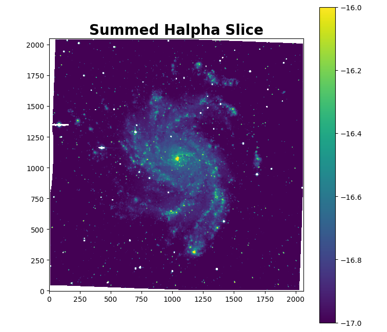
Wavelength of the first slice: 661.25 nm
In the cube directory, under the Luci_outputs subfolder, we have now created a new folder called Slice_Halpha that contains the fits files for each slice and the summed slice. Let’s check out the summed slice!